This is the contract project report submitted to NRCan.
Introduction
In southern New Brunswick, Canada, seasonal flooding takes place around St. John River. According to the report by the Government of New Brunswick, flooding is largely caused by meteorological conditions: thick snowpack remains for a long period each year until the spring thaw when snowmelt runoff flows into rivers, which leads to local overflows [1]. Additionally, the accumulations of rain and the rising temperatures can accelerate snowmelt and surface runoff [1]. Flooding can cause serious damage and inconvenience for citizens’ daily life, and flood susceptibility prediction can help the government and citizens to make response strategies.
Flood modeling has been studied by using a bunch of methods, such as artificial neural networks, support vector machine, and decision-tree-derived machine learning models [2,3]. In addition, hydrological modeling on hexagonal grid meshes has drawn attention among researchers. Previous studies illustrated several key advantages of hexagonal cells compared to traditional square cells in hydrological modeling [4]. Moreover, Discrete Global Grid Systems (DGGS) was increasingly adopted in integrating multi-sources data and solving real-world problems [5]. For example, a DGGS was used to predict flooding risks by adjusting the height above the nearest drainage model, although some of the hydrological variables were computed in a traditional GIS manner before being quantized in the DGGS [6].
This project aimed to apply hexagonal DGGS in flood modeling, with four specific steps:1) quantization of predictor variables in DGGS, 2) derive topographical and hydrological parameters in DGGS, 3) train random forest models across multiple granularities and filter out important predictors, and 4) predict and visualize the flooding susceptibility over the full area.
Study Area and Data Sources
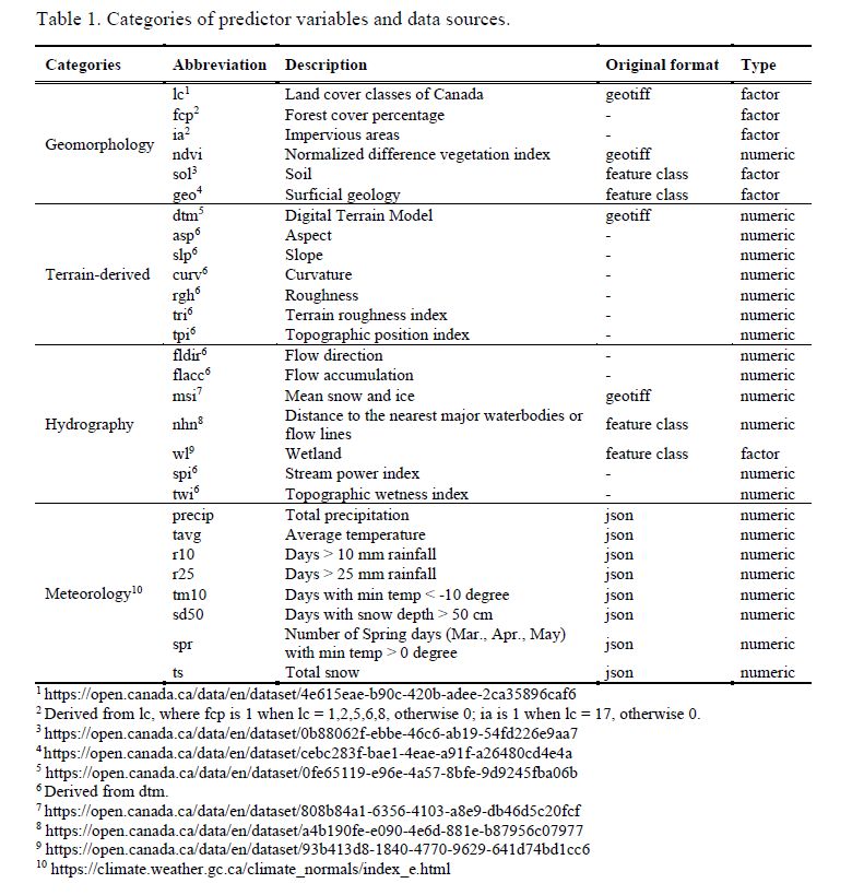
The study area is around 27705 km2, located in southern New Brunswick, and covers the partial drainage basin of St. John River (Figure 1). A total of 2795 sample points were randomly distributed within the study area extent. Their wet and dry attributes, namely flooded and non-flooded, were extracted from the historic record of flood events provided by Open Maps (https://open.canada.ca/data/en/dataset/08b810c2-7c81-40f1-adb1-c32c8a2c9f50). Four categories of 28 predictor variables were included in the modeling: geomorphology, hydrography, meteorology, and terrain-derived variables. Table 1 lists the specific variables under each category and provides their abbreviations, original formats, data types, and data sources. Variable names are referred to as their abbreviations according to Table 1 hereafter.
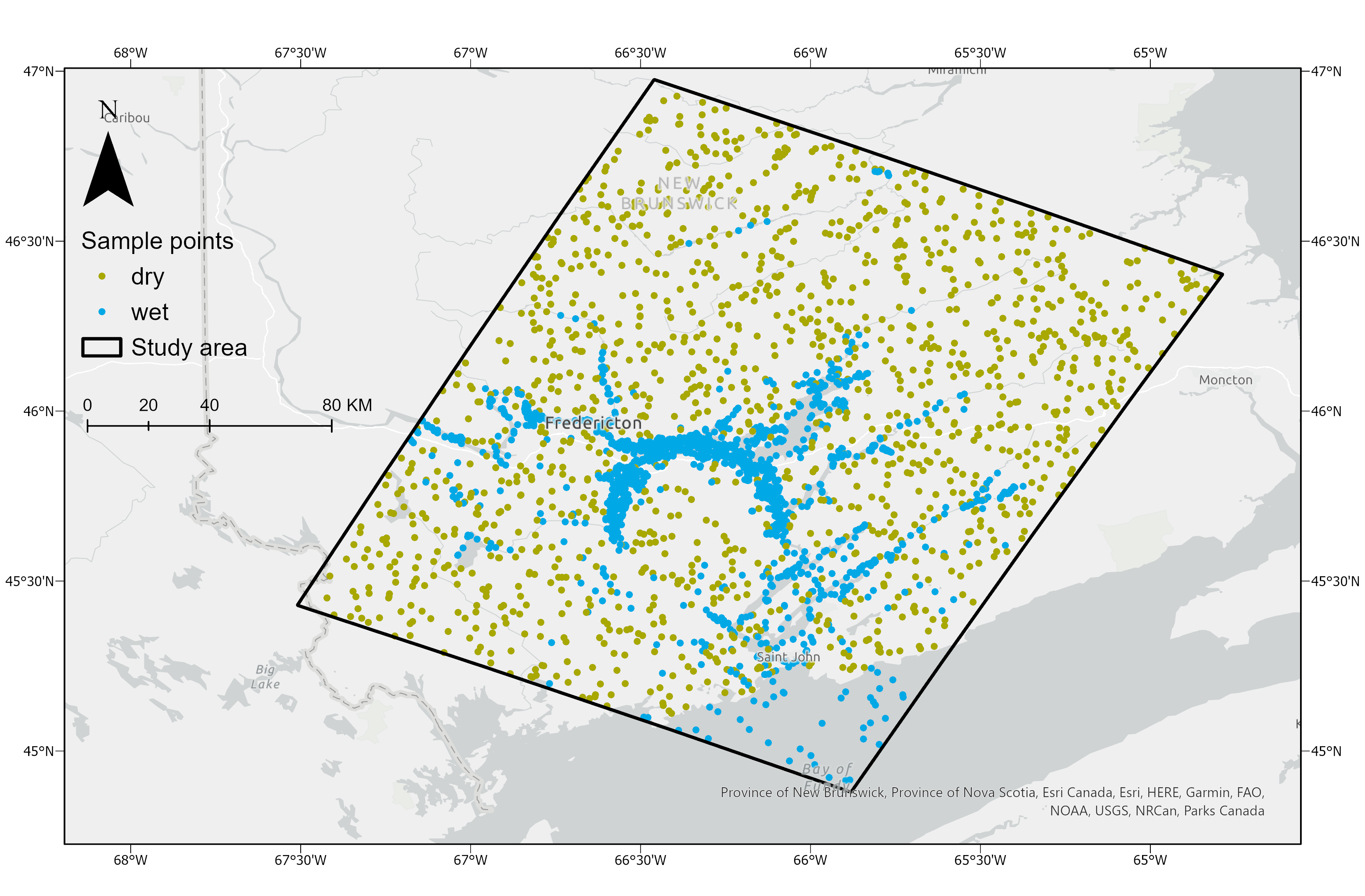 Figure 1. Study area and distribution of dry and wet sample points in New Brunswick, Canada, under the World Geodetic System 1984 (WGS84).
Methodology
DGGS configuration
The DGGS configuration used in this research was the Icosahedral Snyder Equal Area Aperture 3 Hexagonal Grid (ISEA3H). ISEA3H was adopted in several DGGS implementations and used in solving real-world problems [5,7,8]. The DGGS gird was orientated with the latitude of the pole (λ) = 37.6895°, longitude of the pole (φ) = -51.6218°, and azimuth (α) = -72.6482°. Resolution levels 19, 21, and 23 were used in modeling, where the cell sizes were 43885.62, 4876.18, and 541.80 m2 in area, respectively.
Quantization of sample points and predictor variables
Sample points were quantized in the ISEA3H DGGS by converting their longitude-latitude coordinates to cell addresses of nearest cell centroids at levels 19, 21, and 23. Raw datasets in a vector format (sol, geo, and wl) were rasterized before quantization. The quantization process included a series of interpolations over cell centroid locations of sample points. Specifically, predictors with factor (lc, wl, sol, and geo) and numeric (dtm, msi, and ndvi) values were sampled by nearest neighbor interpolation and bilinear interpolation, respectively. Predictors fcp and ia were derived from lc, where fcp = 1 when lc = 1, 2, 5, 6, and 8, and ia = 1 when lc = 17 (otherwise fcp and ia = 0). In terms of nhn, vectors representing major waterbodies and flow lines were firstly rasterized and quantized in DGGS, and hexagonal ring numbers between each quantized sample point to the nearest waterbodies or flow lines were computed as nhn values. The nhn was assigned 0 if the cell was within a waterbody or on a flow line.
Topographical and hydrological parameter production
Topographical predictors including slp, asp, rgh, curv, tri, and tpi were derived from the quantized dtm. Predictors slp and asp were calculated by the Finite-Difference Algorithm (FDA; [9,10]). Predictor rgh was the absolute difference between maximum and minimum elevations within the neighborhood (i.e., six directly connected cells). Predictor curv was calculated as a standard curvature combining both profile and planform curvatures [11]. Topographical indices tri and tpi were generated following their definitions [10,12,13].
Before calculating hydrological parameters, depressions and flat areas were removed following the method proposed by Barnes, et al. [14]. Predictor fldir was computed following the D6 algorithm where the flow of a center cell was always routed to the neighboring cell with the lowest elevation [15], and flacc was then computed based on the flow routing grid. Hydrological indices tri and tpi were generated following their definitions [10,16,17].
Computation of meteorology variables
Climate stations with normal climate data were determined with a 500 m buffer around the study area. Each meteorology variable value of sample points was calculated by Inverse Distance Weighted (IDW) interpolation (power = 2), where the hexagonal ring numbers between quantized sample points and climate stations represented the distance. Predictor spr was the sum of interpolated days with min temp > 0 degree in March, April, and May.
Random forest modeling, evaluation, and prediction
Random forest was used to model and predict the flood susceptibility, where 70% and 30% of sample points were randomly selected for model training and testing, respectively. R library VSURF was used to rank variable importance using training data and predict the flood extent over the full area [18]. Specifically, the important variables were selected by Interpretation Step in VSURF, and variables used to predict flooding were filtered by Prediction Step in VSURF. Three types of models were tested: 1) hydro-geomorphological model (HG) including all geomorphology, terrain-derived, and hydrography predictors (Table 1); 2) HG and precipitation/temperature model (HGPT), which includes all predictors in HG model as well as predictors precip and tavg; and 3) HG and meteorology model (HG8M), which includes all predictors listed in Table 1. Parameters used in the modeling are: ntree = 500, ncores = 8, nfor.thres = 50, nmin = 3, nfor.interp = 25, nsd = 1, nfor.pred = 25, and nmj = 1.
Model performances were evaluated by testing data with three indicators using ROCR library [19]: accuracy (ACC), F-score, and area under the ROC curve (AUC). ACC measures the percentage of samples, both flooding and non-flooding sites, that are correctly classified in the testing datasets [2,3]. F-score and AUC represent the capacity of flooding site identification [2,3].
Models were firstly run with all 28 variables at level 19, and the preliminary results showed that predictors fldir, flacc, twi, and spi were not listed as the top variables. Given the time-consuming computation of flow routing grids at fine resolution levels, these four predictors were excluded from the modeling at levels 21 and 23. Attempts were also given by partitioning the full study area by natural watersheds and combining sub-basin data (all 28 variables) during the modeling. Nonetheless, the results did not outperform the models without fldir, flacc, twi, and spi over the full area. Thus, the following section only reports the tests excluding fldir, flacc, twi, and spi.
Results and Discussion
Important predictors of three types of models at three testing resolutions, ranked by their variable importance, as well as the model performance, were summarized in Table 2. Results showed that dtm was the most important variable across all model types and resolution levels (Table 2). At level 19, lc also showed high importance, especially in HG and HGPT models, followed by nhn, while nhn was generally higher ranked than lc at levels 21 and 23 (Table 2). In addition, at level 21, the geomorphological variable geo had high variable importance following dtm and nhn, although it was less important at the other two testing levels (Table 2).
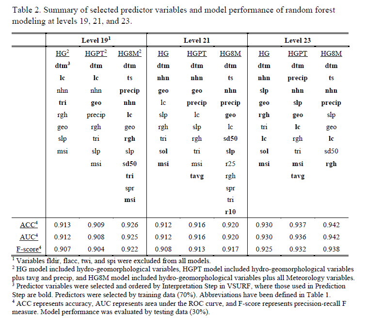
It was also noticed that meteorology variables, precip and ts in particular, were listed as important predictors when being added to the models (e.g., HGPT and HG8M; Table 2). It meant that total precipitation and snow had a strong impact on the occurrence of flooding. Such impact was slightly lower than that of elevations and distances to waterbodies, while higher than the other tested hydro-geomorphological variables.
Models performed well according to three evaluation indicators, where ACC, AUC, and F-score were higher than 0.9 across all model types and resolution levels (Table 2). Generally, models had better performance at finer resolutions with all predictors included in the training process. ACC, AUC, and F-score of HG8M model at level 23 were 0.942, 0.942, and 0.938, respectively (Table 2).
Flood susceptibility prediction
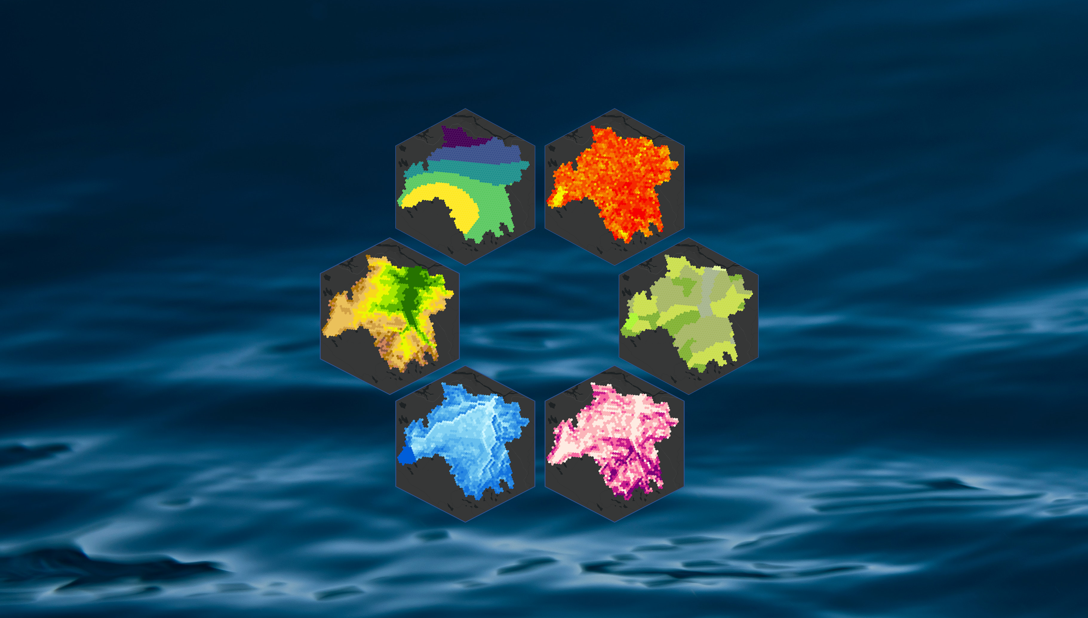
Cell-based flooding events were predicted by three model types at three resolution levels. Figure 2 visualized the predicted flooding sites. Although there were slight differences in the visualized flooding extent in various scenarios, predicted flooding sites were clustered around St. John River and its branches (Figure 1,2).
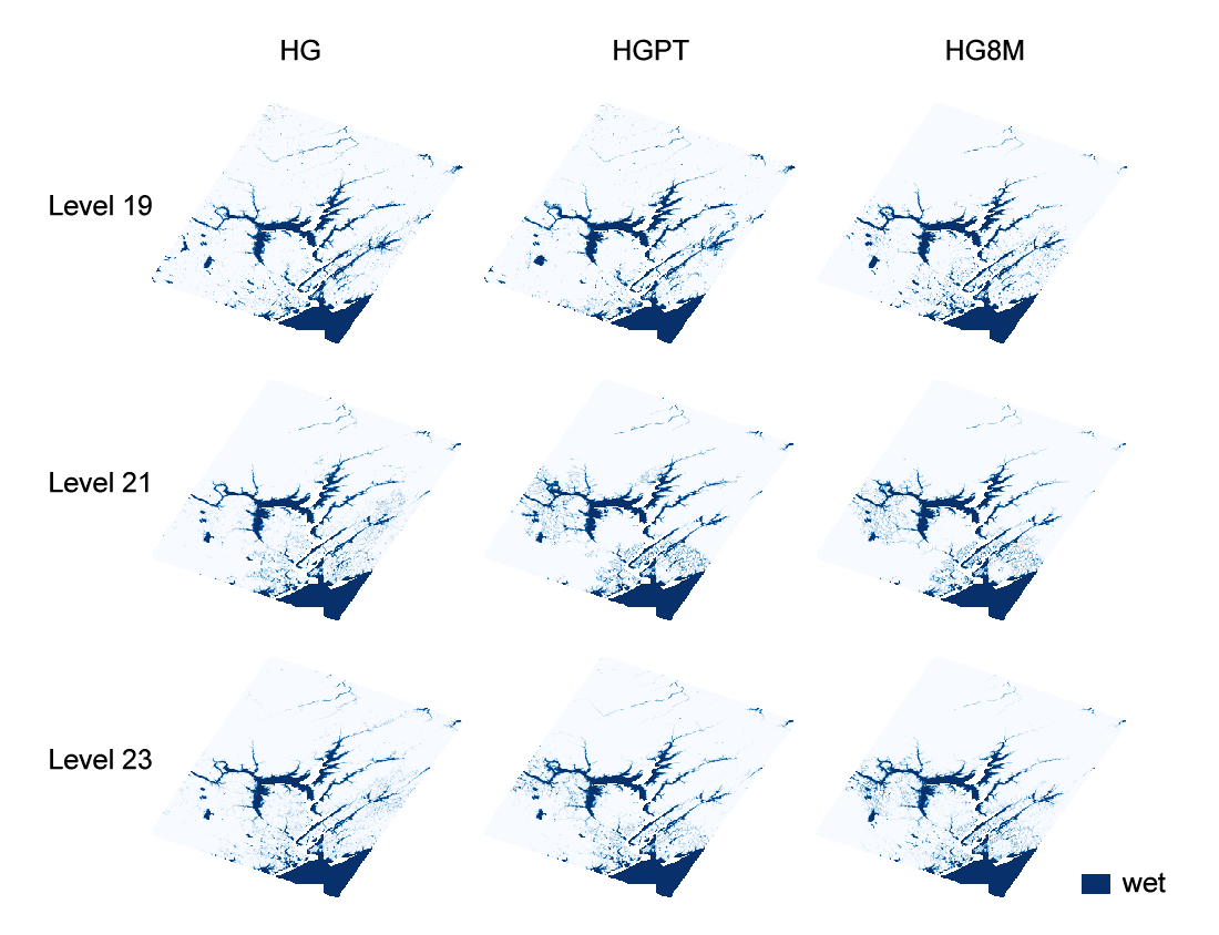 Figure 2. Prediction of the flood extent by HG, HGPT, and HG8M models in the ISEA3H DGGS at levels 19, 21, and 23.
Conclusions, Challenges, and Future Work
This project modeled flood susceptibility using random forest in the ISEA3H DGGS at multiple levels. Four categories of predictor variables were quantized and calculated in a pure DGGS environment and examined in three types of random forest models. Results showed that dtm was the most important variable, generally followed by hydro-geomorphological variables nhn, lc, and geo. Meteorology variables precip and ts showed high importance when being added to the model. Model performance was generally better at finer resolutions with all predictors included. Flood susceptibility was predicted and visualized over the full area.
The major challenge in this project was the amount of computation at fine resolutions. This was especially reflected in the production of flow direction and accumulation. One of the future directions is to parallelize these processes by decomposing the dataset into regular tiles or irregular sub-basins, solving each of them independently, and combining adjacent tiles or sub-basins by joining their edges. Parallel hydrological modeling algorithms proposed by previous studies can be migrated to a hexagonal DGGS environment in the future [20-22]. In addition, more machine learning methods, such as support vector machine, gradient boosting machine, and neural network can be applied and compared at a few more experiment regions.
References
- GNB. Flooding in New Brunswick. Available online: https://www2.gnb.ca/content/gnb/en/departments/elg/environment/content/flood.html (accessed on 27 September 2020).
- Tehrany, M.S.; Jones, S.; Shabani, F. Identifying the essential flood conditioning factors for flood prone area mapping using machine learning techniques. Catena 2019, 175, 174-192, doi:10.1016/j.catena.2018.12.011.
- Zhao, G.; Pang, B.; Xu, Z.; Peng, D.; Xu, L. Assessment of urban flood susceptibility using semi-supervised machine learning model. Sci. Total. Environ. 2019, 659, 940-949, doi:10.1016/j.scitotenv.2018.12.217.
- Liao, C.; Zhou, T.; Xu, D.; Barnes, R.; Bisht, G.; Li, H.-Y.; Tan, Z.; Tesfa, T.; Duan, Z.; Engwirda, D.; et al. Advances in hexagon mesh-based flow direction modeling. Adv. Water Resour. 2022, 160, doi:10.1016/j.advwatres.2021.104099.
- Robertson, C.; Chaudhuri, C.; Hojati, M.; Roberts, S.A. An integrated environmental analytics system (IDEAS) based on a DGGS. ISPRS J. Photogramm. Remote Sens. 2020, 162, 214-228, doi:10.1016/j.isprsjprs.2020.02.009.
- Chaudhuri, C.; Gray, A.; Robertson, C. InundatEd-v1.0: a height above nearest drainage (HAND)-based flood risk modeling system using a discrete global grid system. Geosci. Model Dev. 2021, 14, 3295-3315, doi:10.5194/gmd-14-3295-2021.
- Hojati, M.; Robertson, C. Integrating cellular automata and discrete global grid systems: a case study into wildfire modelling. In Proceedings of the 23rd AGILE Conference on Geographic Information Science, 2020, doi:10.5194/agile-giss-1-6-2020.
- Li, M.; McGrath, H.; Stefanakis, E. Integration of heterogeneous terrain data into Discrete Global Grid Systems. CaGIS 2021, 48, 546-564, doi:10.1080/15230406.2021.1966648.
- Hodgson, M.E. Comparison of angles from surface slope/aspect algorithms. CaGIS 1998, 25, 173-185, doi:10.1559/152304098782383106.
- Li, M.; McGrath, H.; Stefanakis, E. Topographic operations in hexagonal Discrete Global Grid Systems. Int. J. Appl. Earth Obs. Geoinf. 2022, Under Review.
- Goldgof, D.B.; Huang, T.S.; Lee, H. A curvature-based approach to terrain recognition. IEEE Trans. Pattern Anal. Mach. Intell 1989, 11, 1213-1217.
- Guisan, A.; Weiss, S.B.; Weiss, A.D. GLM versus CCA spatial modeling of plant species distribution. Plant Ecol. 1999, 143, 107-122, doi:10.1023/A:1009841519580.
- Riley, S.J.; DeGloria, S.D.; Elliot, R. Index that quantifies topographic heterogeneity intermountain. J. Sci. 1999, 5, 23-27.
- Barnes, R.; Lehman, C.; Mulla, D. Priority-flood: An optimal depression-filling and watershed-labeling algorithm for digital elevation models. Comput. Geosci. 2014, 62, 117-127, doi:10.1016/j.cageo.2013.04.024.
- Wright, J.W. Regular hierarchical surface models: a conceptual model of scale variation in a GIS and its application to hydrological geomorphometry. Doctor of Philosophy, University of Otago, Dunedin, Otago, New Zealand, August 2017.
- Moore, I.D.; Grayson, R.B.; Ladson, A.R. Digital terrain modelling: a review of hydrological, geomorphological, and biological applications. Hydrol. Process. 1991, 5, 3-30, doi:10.1002/hyp.3360050103.
- Beven, K.J.; Kirkby, M.J. A physically based, variable contributing area model of basin hydrology / Un modèle à base physique de zone d’appel variable de l’hydrologie du bassin versant. Hydrology. Sci. Bulletin 1979, 24, 43-69, doi:10.1080/02626667909491834.
- Genuer, R.; Poggi, J.M.; Tuleau-Malot, C. VSURF: an R package for variable selection using random forests. The R Journal 2015, 7, 19-33.
- Sing, T.; Sander, O.; Beerenwinkel, N.; Lengauer, T. ROCR: visualizing classifier performance in R. Bioinformatics 2005, 21, 3940-3941.
- Barnes, R. Parallel non-divergent flow accumulation for trillion cell digital elevation models on desktops or clusters. Environ. Model. Soft. 2017, 92, 202-212, doi:10.1016/j.envsoft.2017.02.022.
- Barnes, R. Parallel Priority-Flood depression filling for trillion cell digital elevation models on desktops or clusters. Comput. Geosci. 2016, 96, 56-68, doi:10.1016/j.cageo.2016.07.001.
- Gong, J.; Xie, J. Extraction of drainage networks from large terrain datasets using high throughput computing. Comput. Geosci. 2009, 35, 337-346, doi:10.1016/j.cageo.2008.09.002.